Parallel Virtual File System (PVFS)
PVFS, the Parallel Virtual File System, is a very high performance filesystem designed for high-bandwidth parallel access to large data files. It's optimized for regular strided access, with different nodes accessing disjoint stripes of data.
Scyld has long supported PVFS, both by providing pre-integrated versions with Scyld ClusterWare and funding the development of specific features.
Writing Programs That Use PVFS
Programs written to use normal UNIX I/O will work fine with PVFS without any changes. Files created this way will be striped according to the file system defaults set at compile time, usually set to 64 Kbytes stripe size and all of the I/O nodes, starting with the first node listed in the .iodtab file. Note that use of UNIX system calls read() and write() result in exactly the data specified being exchanged with the I/O nodes each time the call is made. Large numbers of small accesses performed with these calls will not perform well at all. On the other hand, the buffered routines of the standard I/O library fread() and fwrite() locally buffer small accesses and perform exchanges with the I/O nodes in chunks of at least some minimum size. Utilities such as tar have options (e.g. -block-size) for setting the I/O access size as well. Generally PVFS will perform better with larger buffer sizes.
The setvbuf() call may be used to specify the buffering characteristics of a stream (FILE *) after opening. This must be done before any other operations are performed:
	FILE *fp;
	fp = fopen("foo", "r+");
	setvbuf(fp, NULL, _IOFBF, 256*1024);
/* now we have a 256K buffer and are fully buffering I/O */ |
There is significant overhead in this transparent access both due to data movement through the kernel and due to our user-space client-side daemon (pvfsd). To get around this the PVFS libraries can be used either directly (via the native PVFS calls) or indirectly (through the ROMIO MPI-IO interface or the MDBI interface). In this section we begin by covering how to write and compile programs with the PVFS libraries. Next we cover how to specify the physical distribution of a file and how to set logical partitions. Following this we cover the multi-dimensional block interface (MDBI). Finally, we touch upon the use of ROMIO with PVFS.
In addition to these interfaces, it is important to know how to control the physical distribution of files as well. In the next three sections, we will discuss how to specify the physical partitioning, or striping, of a file, how to set logical partitions on file data, and how the PVFS multi-dimensional block interface can be used.
Preliminaries
When compiling programs to use PVFS, one should include in the source the PVFS include file by:
#include <pvfs.h> |
Finally, it is useful to know that the PVFS interface calls will also operate correctly on standard, non-PVFS, files. This includes the MDBI interface. This can be helpful when debugging code in that it can help isolate application problems from bugs in the PVFS system.
Specifying Striping Parameters
The current physical distribution mechanism used by PVFS is a simple striping scheme. The distribution of data is described with three parameters:
base — The index of the starting I/O node, with 0 being the first node in the file system
pcount — The number of I/O servers on which data will be stored (partitions, a bit of a misnomer)
ssize — Strip size, the size of the contiguous chunks stored on I/O servers
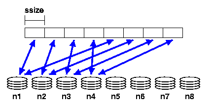
In Figure 1 we show an example where the base node is 0 and the pcount is 4 for a file stored on our example PVFS file system. As you can see, only four of the I/O servers will hold data for this file due to the striping parameters.
Physical distribution is determined when the file is first created. Using pvfs_open(), one can specify these parameters.
pvfs_open(char *pathname, int flag, mode_t mode); pvfs_open(char *pathname, int flag, mode_t mode, struct pvfs_filestat *dist); |
	struct pvfs_filestat
	{
		int base;   /* The first iod node to be used */
		int pcount; /* The number of iod nodes for the file */
		int ssize;  /* stripe size */
		int soff;   /* NOT USED */
		int bsize;  /* NOT USED */
} |
If you wish to obtain information on the physical distribution of a file, use pvfs_ioctl() on an open file descriptor:
pvfs_ioctl(int fd, GETMETA, struct pvfs_filestat *dist); |
Setting a Logical Partition
The PVFS logical partitioning system allows an application programmer to describe the regions of interest in a file and subsequently access those regions in a very efficient manner. Access is more efficient because the PVFS system allows disjoint regions that can be described with a logical partition to be accessed as single units. The alternative would be to perform multiple seek-access operations, which is inferior both due to the number of separate operations and the reduced data movement per operation.
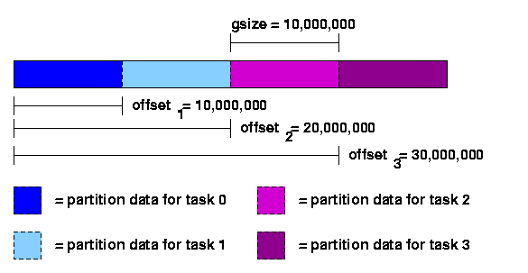
If applicable, logical partitioning can also ease parallel programming by simplifying data access to a shared data set by the tasks of an application. Each task can set up its own logical partition, and once this is done all I/O operations will "see'' only the data for that task.
With the current PVFS partitioning mechanism, partitions are defined with three parameters: offset, group size (gsize), and stride. The offset is the distance in bytes from the beginning of the file to the first byte in the partition. Group size is the number of contiguous bytes included in the partition. Stride is the distance from the beginning of one group of bytes to the next. Figure 2 shows these parameters.
To set the file partition, the program uses a pvfs_ioctl() call. The parameters are as follows: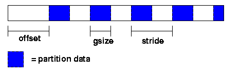
pvfs_ioctl(fd, SETPART, ∂); |
	struct fpart
	{
		int offset;
		int gsize;
		int stride;
		int gstride; /* NOT USED */
		int ngroups; /* NOT USED */
}; |
Alternatively, suppose one wants to allocate the records in a cyclic or "round-robin" manner. In this case the group size would be set to 1000 bytes, the stride would be set to 4000 bytes and the offsets would again be set to access disjoint regions, as shown in Figure 4.
It is important to realize that setting the partition for one task has no effect whatsoever on any other tasks. There is also no reason that the partitions set by each task be distinct; one can overlap the partitions of different tasks if desired. Finally, there is no direct relationship between partitioning and striping for a given file; while it is often desirable to match the partition to the striping of the file, users have the option of selecting any partitioning scheme they desire independent of the striping of a file.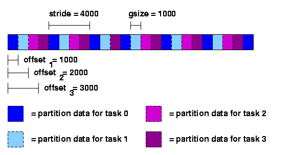
Simple partitioning is useful for one-dimensional data and simple distributions of two-dimensional data. More complex distributions and multi-dimensional data is often more easily partitioned using the multi-dimensional block interface.